SM2007_sims

In this script, I attempt to use calmr’s implementation of SOCR to reproduce some of the figures in Witnauer et al. (2012).

library(ggplot2)
library(magrittr)
library(dplyr)
library(calmr)
theme_set(theme_bw())

The fixed parameters

In Witnauer et al (2012), they set the alphas of cues, contexts, and the US to 0.35, 0.15, and 0.50, respectively. The rate at which associations weaken (k1, here, omega) was set to be 0.22. The weight with which comparison stimuli compete (k2, here, gamma) was set to 0.56. The rate at which the operator switch is learned (k3, here, tau) was set to 0.46. Finally, the strength with which present stimuli are activated (k4, here, rho; see Eq. 4 in their paper) was set to 1.60.

Acquisition

mod <- "SM2007"
des <- data.frame(
  Group = "Acquisition",
  P1 = "100(ctxa)A>(US)/300(ctxa)",
  R1 = FALSE,
  P2 = "1#(ctxa)A/1#(ctxb)A",
  R2 = FALSE
)


pars <- get_parameters(des, model = mod)

pars$alphas[] <- c(.35, .15, .15, .5)
pars$omegas[] <- .22
pars$gammas[] <- .56
pars$rhos[] <- 1.6
pars$taus[] <- .46

pars

## $alphas
##    A ctxa ctxb   US 
## 0.35 0.15 0.15 0.50 
## 
## $lambdas
##    A ctxa ctxb   US 
##    1    1    1    1 
## 
## $omegas
##    A ctxa ctxb   US 
## 0.22 0.22 0.22 0.22 
## 
## $rhos
##    A ctxa ctxb   US 
##  1.6  1.6  1.6  1.6 
## 
## $gammas
##    A ctxa ctxb   US 
## 0.56 0.56 0.56 0.56 
## 
## $taus
##    A ctxa ctxb   US 
## 0.46 0.46 0.46 0.46 
## 
## $order
## [1] 1

m <- run_experiment(des,
  model = mod,
  parameters = pars
)

# Fig 2 A
results(m)$relacts %>%
  filter(s2 == "US" & trial_type == "(ctxa)A>(US)" & phase == "P1") %>%
  mutate(trial = ceiling(trial / block_size)) %>%
  group_by(trial) %>%
  summarise(value = sum(value)) %>%
  ggplot(aes(x = trial, y = value)) +
  geom_line() +
  geom_point()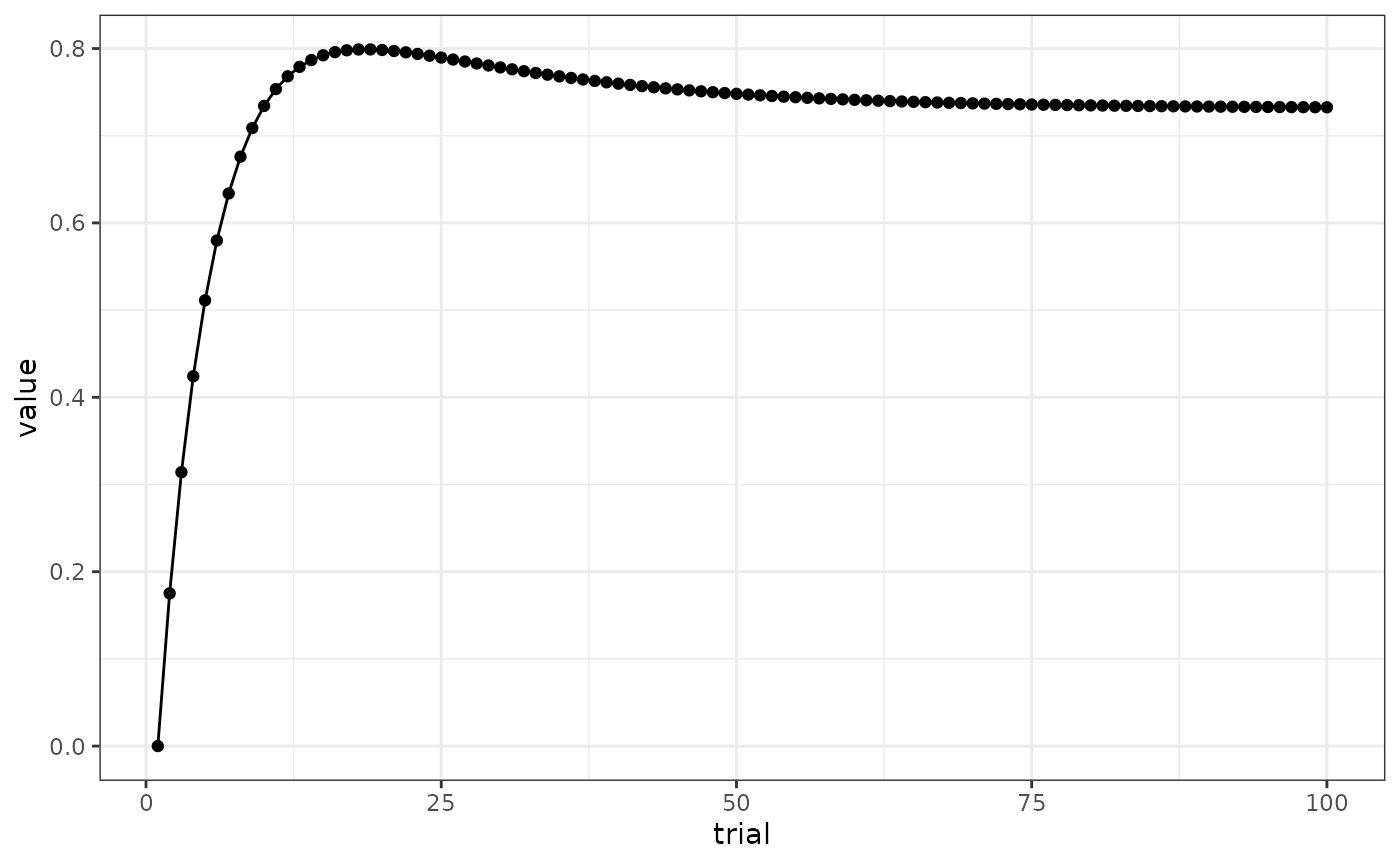

# overall responding levels are higher for calmr

# Fig 2 B
results(m)$relacts %>%
  filter(s2 == "US" & phase == "P2") %>%
  group_by(trial_type) %>%
  summarise(value = sum(value)) %>%
  mutate(trial_type = ifelse(grepl("b", trial_type),
    "Neutral Ctx", "Acquisition Ctx"
  )) %>%
  ggplot(aes(x = trial_type, y = value)) +
  geom_col()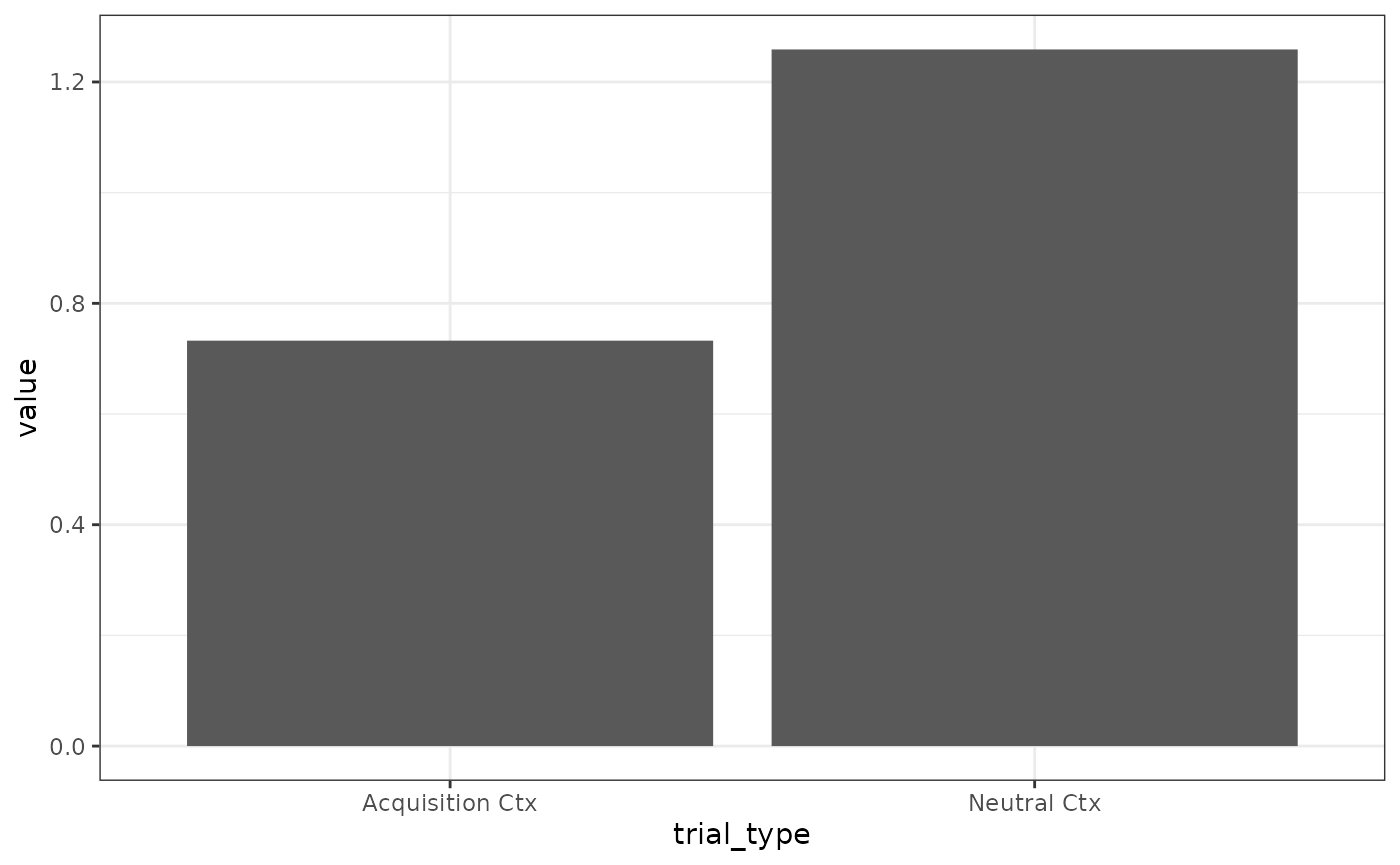

# overall responding levels are higher for calmr

Extinction

des <- data.frame(
  Group = "Extinction",
  P1 = "10(ctxa)A>(US)/30(ctxa)",
  R1 = FALSE,
  P2 = "30(ctxb)A/90(ctxb)",
  R2 = FALSE,
  P3 = "1#(ctxa)A/1#(ctxb)A",
  R3 = FALSE
)

pars <- get_parameters(des, model = mod)
pars$alphas[] <- c(.35, .15, .15, .5)
pars$omegas[] <- .22
pars$gammas[] <- .56
pars$rhos[] <- 1.6
pars$taus[] <- .46

pars

## $alphas
##    A ctxa ctxb   US 
## 0.35 0.15 0.15 0.50 
## 
## $lambdas
##    A ctxa ctxb   US 
##    1    1    1    1 
## 
## $omegas
##    A ctxa ctxb   US 
## 0.22 0.22 0.22 0.22 
## 
## $rhos
##    A ctxa ctxb   US 
##  1.6  1.6  1.6  1.6 
## 
## $gammas
##    A ctxa ctxb   US 
## 0.56 0.56 0.56 0.56 
## 
## $taus
##    A ctxa ctxb   US 
## 0.46 0.46 0.46 0.46 
## 
## $order
## [1] 1

m <- run_experiment(des,
  model = mod,
  parameters = pars
)

# Fig 4 A
results(m)$relacts %>%
  filter(s2 == "US" & trial_type == "(ctxb)A" & phase == "P2") %>%
  mutate(trial = ceiling(trial / block_size)) %>%
  group_by(trial) %>%
  summarise(value = sum(value)) %>%
  ggplot(aes(x = trial, y = value)) +
  geom_line() +
  geom_point()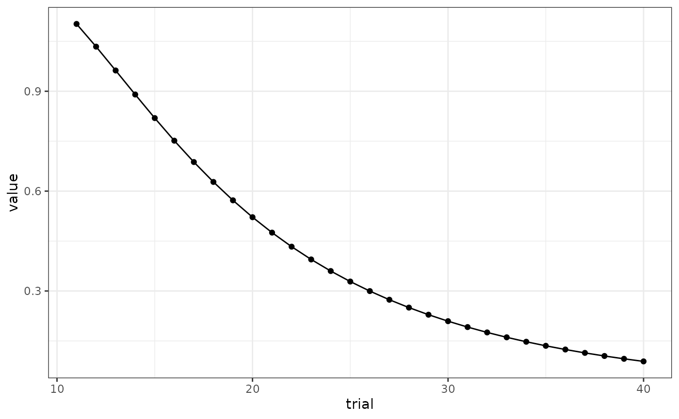

# responding at the beginning of extinction is higher
results(m)$relacts %>%
  filter(s2 == "US" & phase == "P3") %>%
  group_by(trial_type) %>%
  summarise(value = sum(value)) %>%
  mutate(trial_type = ifelse(grepl("b", trial_type),
    "Extinction Ctx", "Acquisition Ctx"
  )) %>%
  ggplot(aes(x = trial_type, y = value)) +
  geom_col() +
  coord_cartesian(ylim = c(0, .4))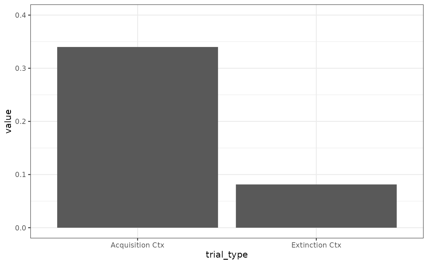

# remarkably similar

Second order conditioning/Conditioned inhibition

des <- data.frame(
  Group = c("Few", "Many"),
  P1 = c(
    "10(ctx)A>(US)/10(ctx)AX/10(ctx)B>(US)/90(ctx)",
    "100(ctx)A>(US)/100(ctx)AX/100(ctx)B>(US)/900(ctx)"
  ),
  R1 = FALSE,
  P2 = "1#(ctx)X/1#(ctx)BX",
  R2 = FALSE
)


pars <- get_parameters(des, model = mod)
pars$alphas[] <- c(.35, .15, .35, .35, .5)
pars$omegas[] <- .22
pars$gammas[] <- .56
pars$rhos[] <- 1.6
pars$taus[] <- .46

m <- run_experiment(des,
  model = mod, parameters = pars
)
# Fig 6

results(m)$relacts %>%
  filter(s2 == "US" & phase == "P2") %>%
  group_by(group, trial_type) %>%
  summarise(value = sum(value)) %>%
  mutate(trial_type = ifelse(grepl("B", trial_type),
    "Summation", "Elemental"
  )) %>%
  ggplot(aes(x = group, y = value, fill = trial_type)) +
  geom_col(position = position_dodge())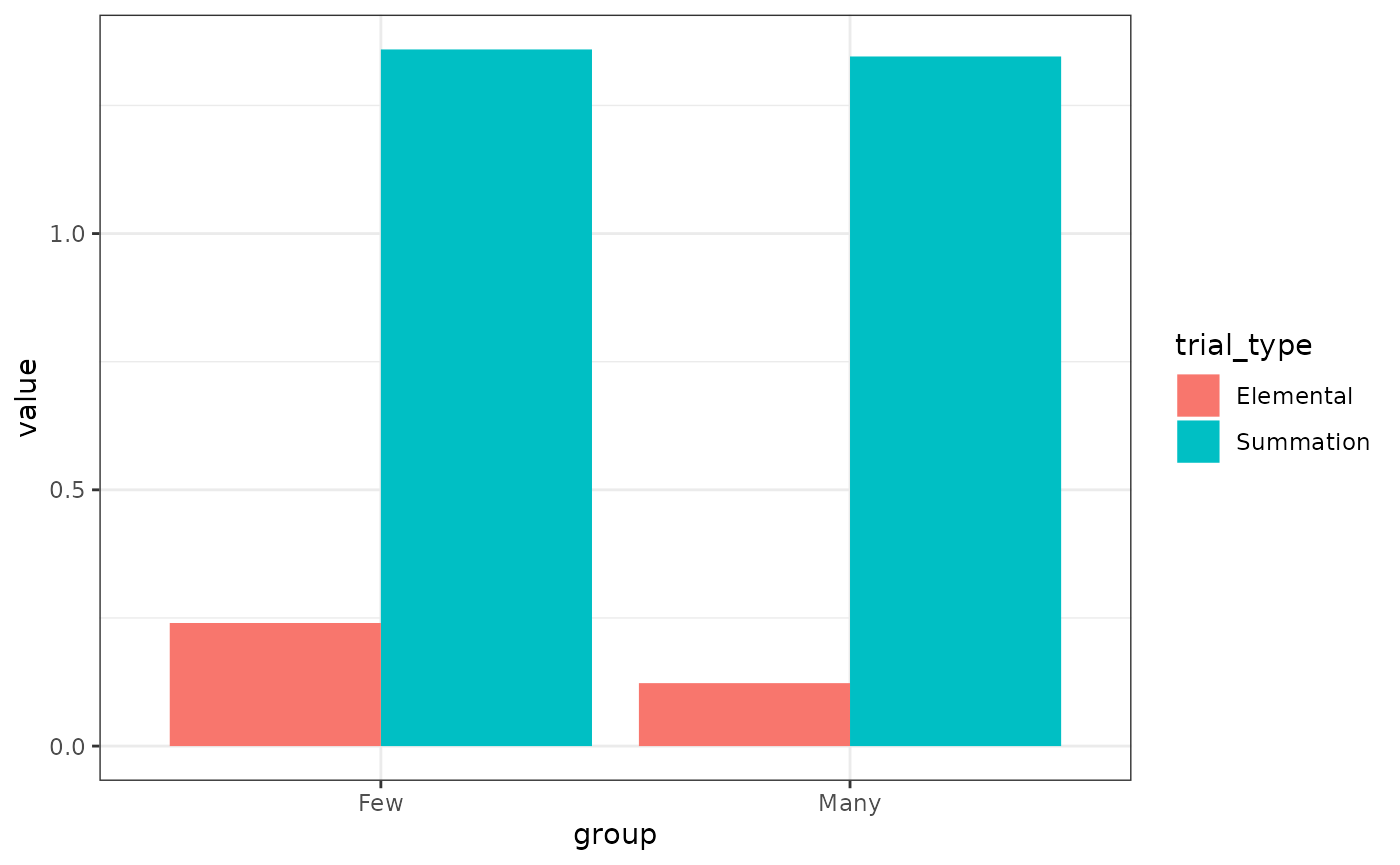

# pretty close, but scales are a little bit off

Blocking

des <- data.frame(
  Group = c(
    "Elemental", "Overshadowing",
    "Blocking", "Recovery From Blocking"
  ),
  P1 = "10(ctx)A>(US)/180(ctx)",
  R1 = FALSE,
  P2 = c(
    "5(ctx)X>(US)/90(ctx)",
    "5(ctx)BX>(US)/90(ctx)",
    "5(ctx)AX>(US)/90(ctx)",
    "5(ctx)AX>(US)/90(ctx)"
  ),
  R2 = FALSE,
  P3 = c(
    "", "", "", # nothing for the first three grups
    "5(ctx)A/90(ctx)"
  ),
  R3 = FALSE,
  P4 = c("1#(ctx)X"),
  R4 = FALSE
)

pars <- get_parameters(des, model = mod)
pars$alphas[] <- c(.35, .15, .35, .35, .5)
pars$omegas[] <- .22
pars$gammas[] <- .56
pars$rhos[] <- 1.6
pars$taus[] <- .46

m <- run_experiment(des,
  model = mod, parameters = pars
)

# Fig 10
results(m)$relacts %>%
  filter(s2 == "US" & phase == "P4") %>%
  group_by(group) %>%
  summarise(value = sum(value)) %>%
  ggplot(aes(x = group, y = value, fill = group)) +
  geom_col()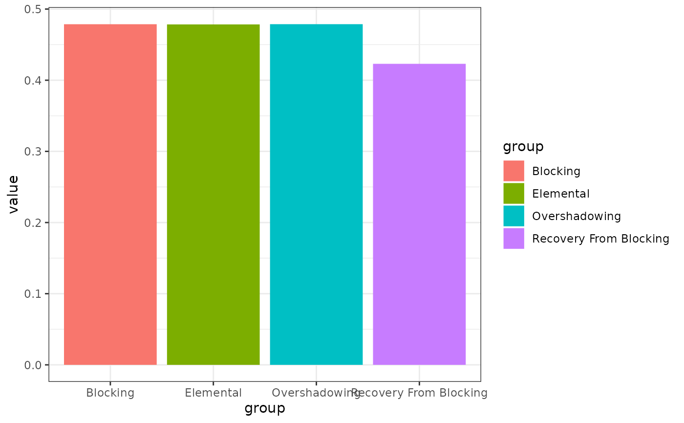

# not even close
# perhaps not enough information to do the simulation?

Unequal associative changes

mod <- "SM2007"
# Gotta love a Miller design
des <- data.frame(
  Group = "Unequal",
  P1 = "100(ctx)X>(US)/100(ctx)XB/100(ctx)XD/100(ctx)A>(US)/100(ctx)C>(US)/1500(ctx)",
  R1 = FALSE,
  P2 = "3(ctx)AB>(US)/9(ctx)",
  R2 = FALSE,
  P3 = c("1#(ctx)AD/1#(ctx)BC"),
  R3 = FALSE
)

pars <- get_parameters(des, model = mod)
pars$alphas[] <- c(.35, .15, .35, .35, .35, .35, .50)
pars$omegas[] <- .22
pars$gammas[] <- .56
pars$rhos[] <- 1.6
pars$taus[] <- .46

m <- run_experiment(des,
  model = mod, parameters = pars
) # takes a bit

# Fig 14
results(m)$relacts %>%
  filter(s2 == "US" & phase == "P3") %>%
  mutate(trial_type = ifelse(grepl("AD", trial_type), "Test AD", "Test BC")) %>%
  group_by(trial_type) %>%
  summarise(value = sum(value)) %>%
  ggplot(aes(x = trial_type, y = value)) +
  geom_point()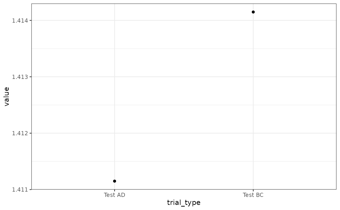

# effect in the right direction,
# but, difference is slightly bigger here

CS Preexposure

des <- data.frame(
  Group = "CSPreexposure",
  P1 = "66(ctx)P/198(ctx)",
  R1 = FALSE,
  P2 = "6(ctx)P>(US)/6(ctx)N>(US)/36(ctx)",
  R2 = FALSE
)

pars <- get_parameters(des, model = mod)
pars$alphas[] <- c(.35, .15, .35, .50)
pars$omegas[] <- .22
pars$gammas[] <- .56
pars$rhos[] <- 1.6
pars$taus[] <- .46

m <- run_experiment(des,
  model = mod, parameters = pars
)

# Fig 14
results(m)$relacts %>%
  filter(s2 == "US" & phase == "P2" & trial_type != "(ctx)") %>%
  mutate(trial = ceiling(trial / block_size)) %>%
  mutate(trial_type = ifelse(grepl("P", trial_type), "Preexposed", "Novel")) %>%
  group_by(trial, trial_type) %>%
  summarise(value = sum(value)) %>%
  ggplot(aes(x = trial, y = value, colour = trial_type)) +
  geom_point() +
  geom_line()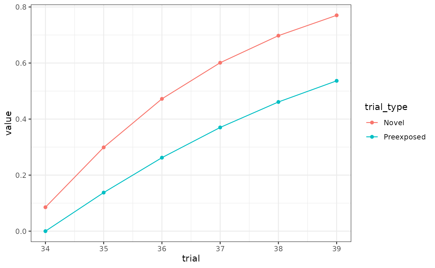

# fairly close in terms of the difference, but scale is off

A final note

All in all, pretty good match between the the calmr implementation and the results reported in the paper. Still, if I were you, reader, I’d use the SM2007 model with caution. If you discover anything, let me know!

References

Witnauer, J. E., Wojick, B. M., Polack, C. W., & Miller, R. R. (2012). Performance factors in associative learning: Assessment of the sometimes competing retrieval model. Learning & Behavior, 40, 347–366. https://doi.org/10.3758/s13420-012-0086-2

Victor Navarro