gganimate | victor

Not long ago I gave a talk about time extensions for HeiDI. As we expand the model to account for quantities (expectations and behavior) across time, it is hard to get some points across with a “fully-revealed” function. Animation not only looks cool, but it also helps in driving some points.

The gganimate package makes (some kinds of) animation fairly trivial. Here’s some R code that generates the following gif.

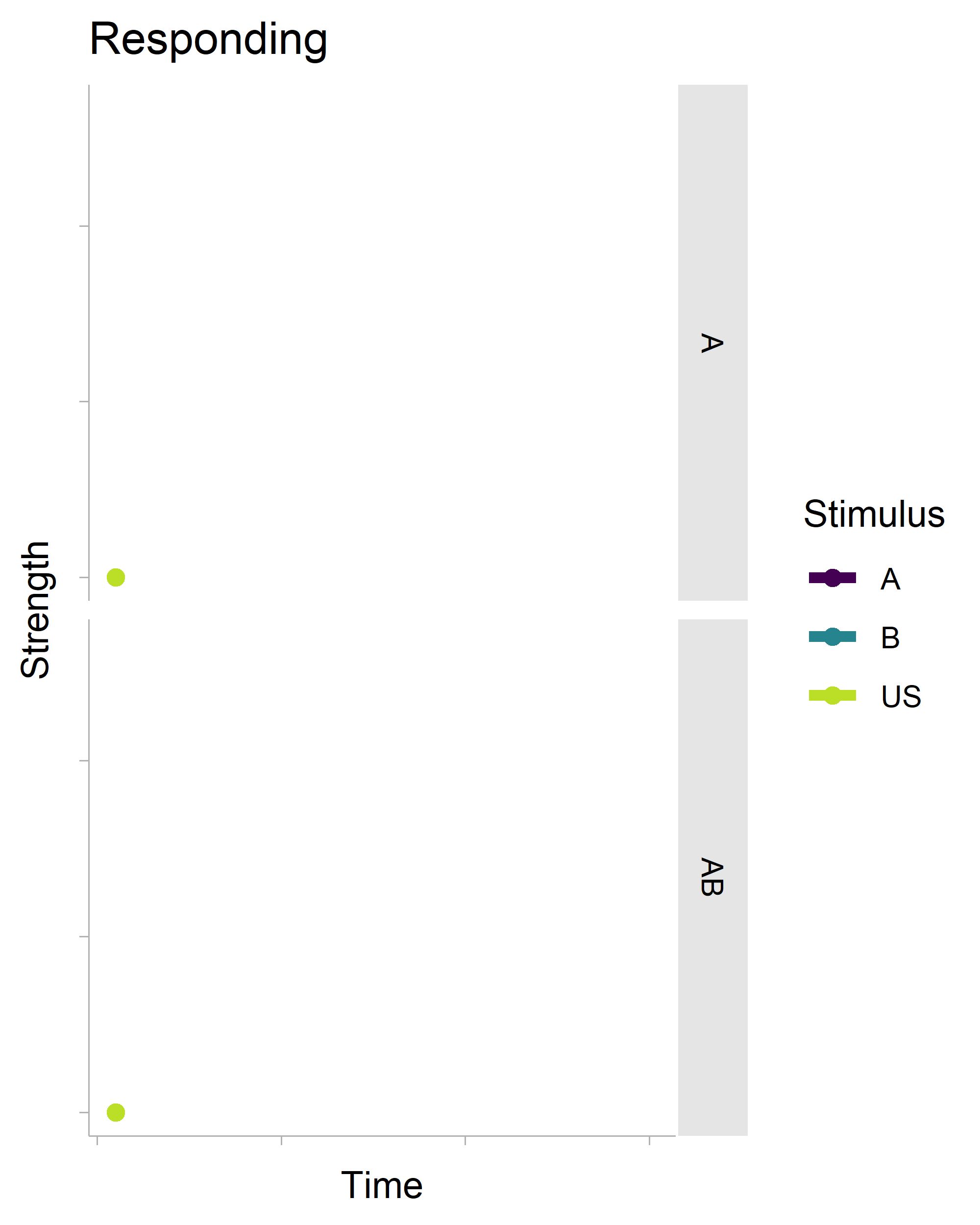
There’s a lot of boilerplate code that generates the data for the plot (it is a full-on model after all), but the critical function is transition_reveal(), which will create an animation based on your x-axis variable. It’s also really smart. Even though there is a geom_point() layer in the non-animated plot, it does not draw every single point in the animation.

require(tidyverse)
require(calmr)
require(gganimate)

source("scripts/time/HD2022_custom.R")
source("scripts/time/helper_functions.R")
source("scripts/time/time_wrapper.R")

scales <- list(
  scale_colour_viridis_d(end = .9),
  scale_fill_viridis_d(end = .9)
)

no_labs <- list(
  theme(axis.text.x = element_blank(), axis.text.y = element_blank())
)

set.seed(2024)
theme_set(tidybayes::theme_tidybayes())

exp <- data.frame(group = "G", P1 = "30A>(US)/30AB", R1 = TRUE)
calm_args <- make_model_args(exp, model = "HD2022")

# these are minimum parameters required to run the model
epochs <- 30
rate <- .1
pwr <- 1
max_cs_alpha <- .4
us_alpha <- .6
other_args <- list(
  alphas = c("A" = max_cs_alpha, "B" = max_cs_alpha, "US" = us_alpha),
  fun_map = c("A" = "A", "B" = "B", "US" = "US"), # functional cs
  fun_alpha = c("A" = max_cs_alpha, "B" = max_cs_alpha, "US" = us_alpha),
  fun_test = list("A" = "A", "AB" = c("A", "B")),
  fun_pots = c("US"),
  min_alpha = 0,
  rate = rate,
  pwr = pwr,
  epochs = epochs,
  test_step = 60,
  sensitivity = 1
)

cs_trace <- power_decay(max_cs_alpha,
  rate = rate,
  pwr = pwr, times = 10
)

off_trace <- power_decay(min(cs_trace),
  rate = rate * 3,
  pwr = pwr, times = 10 + 1
)[2:(10 + 1)]
cs_alpha <- cs_trace[10]

manual_alphas <- array(0,
  dim = c(2, other_args$epochs),
  dimnames = list(c("A", "B"), 1:other_args$epochs)
)
manual_alphas["A", 11:30] <- c(cs_trace, off_trace)
manual_alphas["B", 11:30] <- c(cs_trace, off_trace)

other_args$manual_alphas <- manual_alphas
other_args$calm_alphas <- c("A" = cs_alpha, "B" = cs_alpha, "US" = us_alpha)

mod <- time_wrapper(other_args, calm_args)
# parse_mod

rs <- parse_mod(mod, "rs") %>%
  filter(s2 == "US") %>%
  mutate(value = ifelse(is.na(value), 0, value))

rs_plot <- rs %>% ggplot(aes(x = epoch, y = value, colour = s1)) +
  geom_line(linewidth = 1.5) +
  geom_point(size = 2) +
  scales +
  no_labs +
  labs(
    x = "Time", y = "Strength",
    title = "Responding", colour = "Stimulus"
  ) +
  facet_grid(trial_type ~ .) +
  transition_reveal(epoch)

rs_anim <- animate(rs_plot,
  renderer = gifski_renderer(),
  height = 5, width = 4, units = "in", res = 500,
  duration = 10
)

anim_save("everything_rs.gif", rs_anim)

P.s. The bits of code that extend HeiDI will be released on OSF soon^tm

Enjoy Reading This Article?